Abstract
Street-level imagery platforms such as Mapillary offer a route to measuring urban infrastructure — sidewalk presence, road surface quality, street lighting, vegetation, building density — at a scale and cost no manual survey can match, in a country, India, where no verified prior work has applied this method at the street level. But the imagery itself is not a random sample of the urban fabric: coverage is contributed unevenly, correlated with population density, road importance, and plausibly the same socioeconomic factors infrastructure quality itself correlates with. A model trained and evaluated only where imagery happens to exist risks measuring "infrastructure where people happened to drive with a camera," not infrastructure. UrbanLens India asks two questions: (1) can street-level computer vision measure infrastructure attributes in Indian cities, and (2) how biased is that measurement by uneven imagery coverage, and can classical missing-data correction (inverse-propensity weighting, post-stratification) recover an unbiased estimate?
This paper reports where the project actually stands, honestly. It does not report a completed empirical study of Indian cities' infrastructure — no Mapillary API token has yet been obtained, so no imagery coverage has been measured, no street images labeled, and no vision model trained or evaluated. What it does report is a completed methodological validation: a controlled masking experiment, built on a real 1,034,146-point OpenStreetMap road network across 9 Indian cities and real WorldPop/VIIRS/GHSL covariates at every point, in which a known ground truth is simulated so IPW and post-stratification can be graded against it directly. Under a missing-completely-at-random (MCAR) mask, naive estimation is already accurate (0.05% error) as expected. Under a missing-at-random-like (MAR-like) mask mimicking this project's actual coverage-bias hypothesis, the naive covered-only estimate is biased by 20.89%; a gradient-boosted-propensity IPW estimator recovers to 2.29% error, logistic IPW to 8.24%, and post-stratification to 10.78%. This is real evidence the correction machinery works when the coverage mechanism is roughly as hypothesized — but it is evidence about the method, not India's actual infrastructure or coverage bias, and the paper is explicit throughout about that boundary. The full measurement pipeline (src/coverage/, src/vision/, src/eval/, src/bias/) is built, unit-tested against synthetic fixtures, and ready to run against real imagery the moment a Mapillary developer token is obtained.
Introduction
Two gaps motivate this project, both surfaced by a source-verified literature review (docs/literature_review.md) rather than assumed. First: no verified paper measures street-level infrastructure attributes in Indian cities specifically. Satellite-based slum mapping in India exists and is well established — CNN transfer learning distinguishes slum from non-slum built form in Mumbai at 90–94% accuracy (Wurm et al.), and U-Net segmentation does the same across five Maharashtra cities using Sentinel-2 imagery — but satellite resolution cannot see a sidewalk, a lamp post, or a road surface. Street-level computer vision has been applied to exactly these attributes elsewhere: Streetscore-style perceptual scoring (Naik et al. 2014) and large-scale demographic proxying (Gebru et al. 2017) in the US, the Green View Index for street vegetation (Li et al. 2015), and Project Sidewalk's deep-learning sidewalk-accessibility model (Weld et al. 2019). Mapillary specifically has been used for global road-surface classification (Randhawa et al. 2024/2025), which explicitly notes uneven coverage "including in India" without a city-level breakdown. None of this literature closes the loop for Indian street infrastructure specifically — this project's first target, still open pending real imagery access.
Second: no verified paper bridges classical missing-data correction — IPW (Rubin 1976's MCAR/MAR/MNAR taxonomy; Seaman & White 2013's IPW review; Little 1993's post-stratification theory) — to street-imagery coverage bias specifically. The closest work quantifies the existence of the problem (a 2024/2025 Computers, Environment and Urban Systems study finds street-view imagery reaches only 62% of buildings, with facade coverage averaging 12.4%; a parallel Nature Scientific Data effort documents sparse crowdsourced Mapillary coverage across Africa) without applying a correction. UrbanLens India's second contribution is applying IPW and post-stratification to this exact setting, reported here partially validated: the masking experiment below demonstrates the correction machinery recovers a known ground truth under a realistic simulated coverage mechanism, but not yet on real measured coverage and real infrastructure labels, because those do not exist yet — a real, current limitation reported honestly rather than glossed over.
The rest of this paper is organized around the project's full intended pipeline — Data, Imagery Coverage, Infrastructure Labels, Vision Models, Cross-City Generalization, Coverage Bias, Correction Methods — describing, for each stage, what has been built, what is real, and what is pending. The Results section reports only the one experiment that is complete: the masking experiment. Limitations and Ethics sections are written with the same standard of honesty that governs the rest of the project.
Related Work
Street-level computer vision for urban measurement. Naik, Philipoom, Raskar & Hidalgo (2014, CVPR Workshops) trained an SVM/GIST "Streetscore" model on crowd-labeled perceived safety across roughly one million Google Street View images from 21 US cities, establishing that a physical or perceptual urban attribute can be derived from street imagery at scale. Gebru, Krause, Wang, Chen, Deng, Lieberman Aiden & Fei-Fei (2017, PNAS) detected car make/model across 50 million Street View images in 200 US cities and showed the resulting statistics predict income, race, education, and voting patterns — evidence that street-imagery features carry real socioeconomic signal, the logic this project applies to infrastructure instead of vehicles. MIT's Senseable City Lab (Li et al.) validated Street-View-derived urban-form metrics (building height, street enclosure) against independent ground truth, a template this project would follow once real predictions exist. Li, Zhang, Li et al. (2015, Landscape and Urban Planning) established the Green View Index — percent-of-frame greenery — as the standard street-level vegetation metric, direct ancestor of this project's ordinal vegetation attribute. Weld, Jang, Zeng, Kim, Guo & Froehlich (2019, ASSETS '19) trained the first deep-learning sidewalk-accessibility model on 300,000+ crowdsourced Project Sidewalk labels — the closest precedent for this project's sidewalk-presence attribute.
Mapillary-specific work. Randhawa, Aygün, Randhawa, Herfort, Lautenbach & Zipf (2024/2025, arXiv:2410.19874) is the closest methodological analog: a Swin-Transformer model classifying paved/unpaved road surface from 105 million Mapillary images globally (F1 91–97% vs. OSM tags), explicitly noting "Japan, Thailand and some parts of India showed good coverage while Pakistan, Iran and Indonesia showed notably sparse coverage" — the only documented India-coverage data point found, with no city-level granularity, precisely the gap src/coverage/check_mapillary_coverage.py is built to fill. A Nature Scientific Data (2025) ~200,000-image labeled Mapillary road-surface dataset for Africa independently documents sparse Global-South Mapillary coverage. Hou, Quintana, Khomiakov, Yap, Ouyang, Ito, Wang, Zhao & Biljecki (2024, ISPRS J. Photogrammetry and Remote Sensing) assembled "Global Streetscapes" (10M images, Mapillary + KartaView, 688 cities, 210 countries) as a candidate external cross-city benchmark. Warburg et al. (2020, CVPR) introduced the Mapillary Street-Level Sequences (MSLS) place-recognition benchmark (1.6M images).
India and the Global South. Wurm, Stark, Zhu, Weigand & Taubenböck (Habitat International) reached 90–94% accuracy distinguishing slum/non-slum built form in Mumbai via transfer-learning CNNs on satellite imagery; a 2023 IEEE paper applied U-Net segmentation to Sentinel-2 imagery across five Maharashtra cities for the same task; separate uncertainty-quantification work (including Ahmedabad) treats spatial uncertainty in Global-South slum-boundary delineation as a first-class output, a parallel this project follows for both CV-prediction confidence and bias-correction uncertainty once real numbers exist. All of this is satellite-resolution; no verified paper applies street-level CV to infrastructure attributes in Indian cities specifically — the gap docs/literature_review.md flags and this project's clearest claim to novelty.
Geographic and dataset bias. Shankar, Halpern, Breck, Atwood, Wilson & Sculley (2017, NeurIPS Workshop on ML for the Developing World) is the canonical citation establishing ImageNet/Open Images are ~33% US-sourced and 60% from six North American/European countries — the skew this project's premise generalizes to street imagery. de Vries, Misra, Wang & van der Maaten (2019, CVPR Workshops) extend this to income-conditioned appearance shift (Dollar Street, 54 countries), relevant to the cross-city generalization risk the split strategies below are designed to surface. A 2024/2025 Computers, Environment and Urban Systems paper, "Coverage and Bias of Street View Imagery in Mapping the Urban Environment," is the closest quantitative precedent: SVI reaches only 62% of buildings in its case study, with facade coverage averaging 12.4%, position- and building-type-dependent.
Missing-data and reweighting. Rubin (1976, Biometrika) introduces the MCAR/MAR/MNAR taxonomy used throughout to frame coverage as a missing-data problem. Little (1993, JASA 88(423)) is the theoretical reference for the post-stratified estimator in src/bias/reweighting.py. Seaman & White (2013, Statistical Methods in Medical Research) survey IPW and its sensitivity to propensity misspecification — the caveat directly informing the masking-experiment design and this project's weight truncation/stabilization. No verified paper applies IPW or post-stratification specifically to remote-sensing or crowdsourced geospatial coverage bias — this combination is a genuinely novel application, stated as a contribution, not restated as established practice.
Spatial leakage and generalization. Ploton, Mortier, Réjou-Méchain, Barbier et al. (2020, Nature Communications 11:4540) is the canonical demonstration that spatial autocorrelation inflates apparent model performance: non-spatial cross-validation of a forest-biomass model shows >50% variance explained, collapsing to near-zero true predictive power once spatially blocked — this directly motivates the spatial-block and city-holdout splits in src/eval/splits.py. Karasiak et al. (Machine Learning, Springer) confirm the same spatial-dependence effect inflates remote-sensing accuracy more broadly. A 2022 Computers, Environment and Urban Systems paper, "Fair train-test split in machine learning," proposes the grid-based spatial-blocking methodology adopted directly here.
Data
City selection. The candidate pool spans 14 Indian cities selected by stratified sampling across region (North, West, South, East, Central — four of India's five broad zones populated; Northeast omitted for lack of any documented Mapillary presence to check, flagged rather than silently dropped), population tier (megacity >4M, large 1–4M, mid-size 0.3–1M using 2011 Census of India city-proper populations, from Mumbai at 12,442,373 down to Mysuru at 920,550), and economic tier (a coarse, qualitative state-level grouping from the RBI's Handbook of Statistics on Indian States; exact per-capita NSDP figures were not machine-extractable from the RBI's PDF handbook, so the tier label is a documented qualitative placeholder, not a fabricated number). Crucially, this selection happened before any imagery-coverage check: a sample chosen for good Mapillary coverage would make the coverage-bias question unanswerable by construction, since the study would only ever observe the well-covered case. The project's own protocol commits to keeping at least one low-coverage, low-economic-tier city in the eventual N=4 final study sample even if its measured coverage turns out to be poor, because a coverage-bias study that discards poorly-covered cities cannot say anything about coverage bias.
Road-network universe. Of the 14-city pool, 9 cities currently have a fetched OpenStreetMap road network (ahmedabad, bengaluru, bhopal, coimbatore, mysuru, nagpur, patna, pune, ranchi), retrieved via the Overpass API under OSM's ODbL license, with query text, retrieval timestamp, and OSM version recorded per city for reproducibility. For each city, the sampling area is a fixed 6km-radius circle around the city center (radius_m: 6000 in every manifest), independent of city population or footprint — a deliberate choice, not an oversight. Without a fixed radius, sampling would implicitly cover more physical area for a megacity than a mid-size city, confounding "city size" with "sampling extent" in every downstream comparison; a fixed-radius urban core instead makes population and economic tier the actual varying factors under comparison. Within that radius, every OSM highway-classed road edge is resampled into points spaced 50 meters apart (src/coverage/build_road_universe.py), producing the coverage-analysis spatial unit universe: 1,034,197 points across the 9 cities (data/interim/road_universe_meta.json), built independent of where imagery happens to exist — the same "select the universe before checking coverage" discipline as city selection, applied one level down.
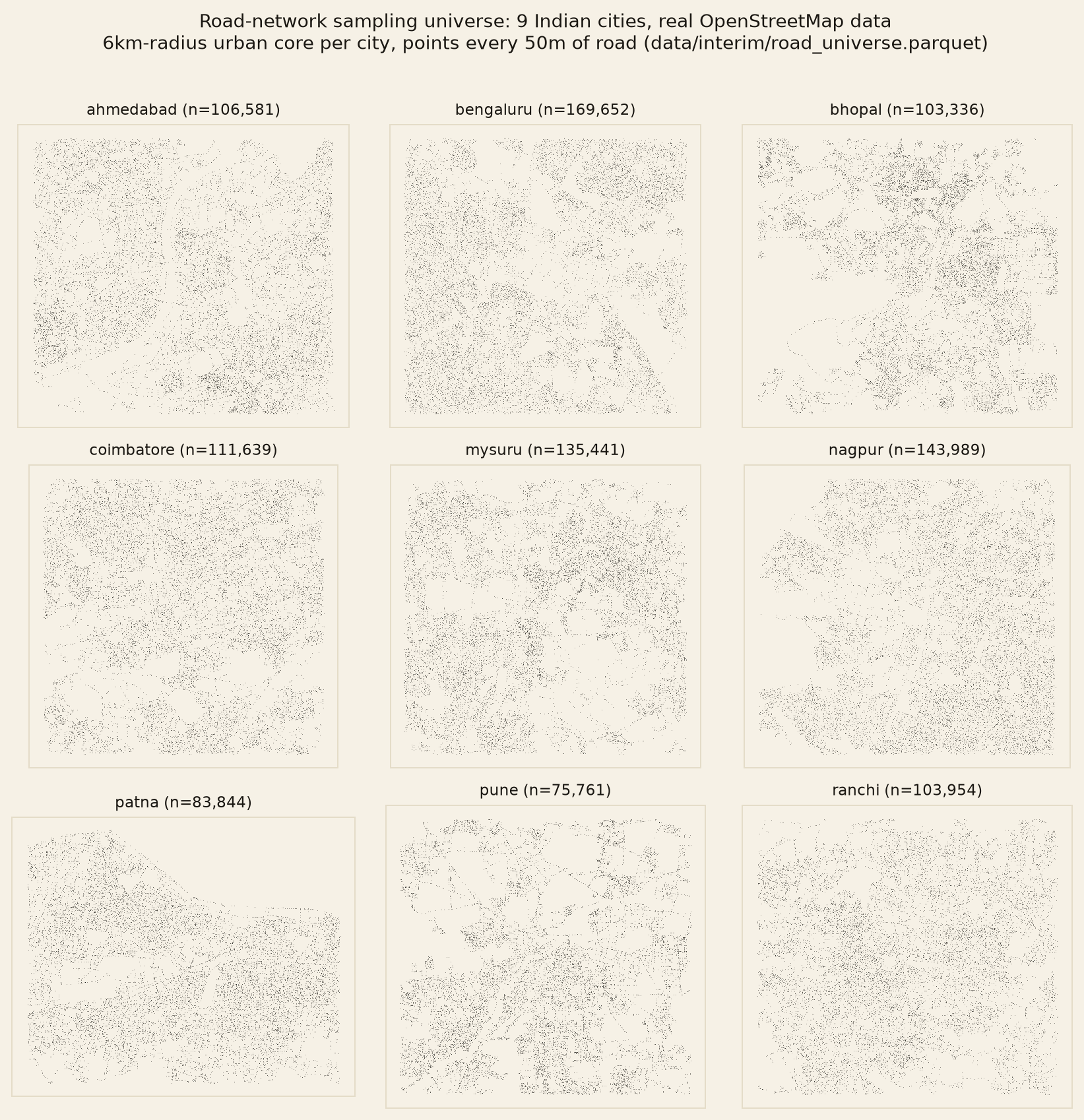
The visible differences in shape across cities are real geography, not sampling artifacts — Patna's network, for instance, is truncated along the Ganges riverbank within its 6km radius.
Geospatial covariates. Three covariates are joined onto every road-universe point (src/coverage/fetch_covariates.py, data/interim/covariates.parquet, 1,034,197 rows, near-100% non-null): WorldPop population density, VIIRS-consistent nighttime-lights radiance, and GHSL built-up surface area. Each required a documented routing change from the original plan, recorded honestly rather than silently substituted. WorldPop is used at 1km resolution rather than the planned 100m — the 100m national GeoTIFF (~1.8GB) was empirically throttled to a few KB/s over WorldPop's HTTPS endpoint, while the same tree served over FTP at >1MB/s, so the 1km product (18MB) was fetched that way; a real, documented resolution downgrade. Nighttime lights come not from the official NOAA/NCEI distribution (an OIDC login wall with no available credentials) or Google Earth Engine (unavailable in this environment) but from Chen, Wang & Zhang (2024, Scientific Data), "A global annual simulated VIIRS nighttime light dataset from 1992 to 2023" (DOI 10.6084/m9.figshare.22262545), using its 2023 layer, which per the source paper's own methodology is the real annual VIIRS DNB composite for that year (only pre-2012 years are a DMSP-based reconstruction, not used here) — real, peer-reviewed, DOI-citable data, substituted for a documented empirical reason, not fabricated. GHSL built-up surface (GHS-BUILT-S R2023A, epoch 2020, 100m) was obtained as planned, fetched as five Mollweide tiles located by a real spatial join against JRC's tile-grid shapefile rather than a whole-globe download or a hardcoded guess.
Imagery Coverage
The instrument for measuring real Mapillary coverage is fully implemented at src/coverage/check_mapillary_coverage.py. For each city, it queries the Mapillary Graph API v4 for every image within that city's 6km sampling radius (src/data/mapillary_client.py), then for every road-universe point computes the distance to the nearest returned image via a cKDTree over a local equirectangular projection (adequate at the under-10km city scale used here, avoiding a pyproj dependency). A road point is marked covered if an image was captured within a 25-meter snap radius; image count within that radius and capture-date range are also recorded, so coverage can be characterized as density and recency, not just binary presence. The cheap primary tool for coverage density without downloading imagery is Mapillary's coverage-tile endpoint (50,000 requests/day budget, never touching raw image bytes); full per-image bbox queries (each capped at ~1.1km × 1.1km at Indian latitudes, 2,000 images/request) are used where finer snap-radius matching is needed.
This script has not been run. It requires a MAPILLARY_TOKEN — a free developer client token from mapillary.com/developer — not yet provided to this project; the script fails loudly rather than substituting a placeholder if unset. This is the single blocking dependency for the entire empirical half of the project: make coverage (this script), make labels (sampling the labeling queue from measured coverage), make train (fitting vision baselines against real labeled images), and make bias-study (real propensity models, real IPW/post-stratification) all cascade from it in that order. Once a token exists, make coverage would produce data/interim/coverage/coverage_universe.parquet — one row per road-universe point with a real covered boolean, image count, and capture-date range — and a per-city coverage summary, the actual empirical answer to "how uneven is Mapillary coverage across these 9 Indian cities" that this paper does not yet have and does not fabricate.
Infrastructure Labels
The annotation protocol (docs/annotation_protocol.md, machine-readable schema at data/labels/schema.json) defines five target attributes, each with direct literature precedent and plausibly answerable from a single street-level frame without specialized sensors: sidewalk presence; road surface type (paved/unpaved, following the binary used in Randhawa et al.'s global Mapillary road-surface study); street vegetation (a coarse three-level ordinal simplification of the Green View Index — low/medium/high, since pixel-level GVI would require segmentation labels beyond this project's first-pass labeling budget); street lighting presence; and immediate building frontage density (a frame-visible proxy for building density, scoped away from a lot-coverage-ratio estimate that would need parcel data this project lacks).
This is a deliberate subset of the full spec's attribute list. Road width, crosswalk-level detail, and drainage indicators were considered and explicitly not attempted: a single monocular image cannot reliably support metric width estimation without stereo or LiDAR, and informal review of sample Indian streetscape imagery found crosswalk and drainage visibility inconsistent enough that a protocol for them would produce labels nobody could apply consistently — cutting them is the honest choice the project's own standard demands (do not pretend every attribute can be reliably inferred from a photograph), not a completeness failure.
Every attribute shares the same five-way label set: positive, negative, uncertain (visible but genuinely ambiguous even to a careful annotator), not_visible (camera geometry or obstruction excludes the relevant part of the scene), and unusable (the image itself is unusable — night imagery, motion blur, heavy occlusion, adverse weather, wrong camera orientation, unusual road geometry, active construction, a corrupted frame — in which case no attribute on that image gets a real label). The protocol reserves a fixed 10% overlap sample labeled independently by two annotators, with Cohen's kappa computed per attribute by src/labeling/agreement.py. No labeling has occurred yet — blocked on the same missing Mapillary token as the coverage check, since there is no imagery to label until make coverage and make labels have run. Inter-rater agreement is therefore also not yet measured; this paper makes no claim about label reliability beyond the protocol's design. This is currently a single-researcher project, so "two annotators" is a design intent, not a guarantee: docs/annotation_protocol.md flags explicitly that if the eventual overlap sample is labeled by the same person twice, the resulting kappa measures intra-rater consistency, not inter-rater reliability, and whichever is actually true must be reported as such once real numbers exist, not glossed as "inter-rater agreement" by default.
Vision Models
Three baselines are implemented in src/vision/, following the project's required progression from cheapest to most adaptive. All three share a single encoder choice, CLIP ViT-B/32 (OpenAI pretrained weights, via open_clip), justified in src/vision/embeddings.py on three grounds: it serves all three baseline roles (frozen features for a linear probe, a fine-tunable backbone, and zero-shot classification via its paired text encoder) from one cached embedding format; at roughly 151M parameters and a 338MB checkpoint it runs a CPU forward pass in well under a second per image with no GPU required, matching the project's tractability constraint; and it has direct precedent in the zero-shot vision-language literature this project draws on. A plain ImageNet ResNet18 would be cheaper still but buys nothing for the zero-shot baseline, which specifically needs a joint image/text embedding space.
Zero-shot CLIP (zero_shot_clip.py) compares an image embedding against prompt-ensembled positive/negative text-prompt embeddings, applied only where a short literal caption plausibly describes the attribute's states — sidewalk presence, road surface type, and street lighting — and explicitly not to street vegetation (a three-level ordinal, not a clean binary) or building frontage density (a fuzzier, composition-dependent judgment CLIP's largely object/scene-level pretraining is unlikely to capture well, and the attribute the protocol itself flags as most ambiguous). Linear probe (baseline_linear_probe.py) fits one independent scikit-learn LogisticRegression per attribute on frozen cached CLIP embeddings — five independent binary classifiers, since attributes are not mutually exclusive. Fine-tuned classifier (finetune_classifier.py) trains a linear head on top of the CLIP visual encoder end-to-end, with a masked binary cross-entropy loss computed elementwise so a partially-masked image still contributes gradient for its labeled attributes only. Running both a frozen probe and an end-to-end fine-tune separates "how good are off-the-shelf CLIP features here" from "does adapting the encoder to Indian street scenes help."
No training has occurred against real data. Every script above defaults to a smoke-test mode against a tiny synthetic image fixture with a random-initialized encoder, so pipeline mechanics — caching, masking logic, per-attribute fitting, checkpoint writing — are verified without a network dependency or real labeled data; none of those numbers should be, or are, read as a research result. Real runs require --labels-csv pointing at real annotation output, which does not exist yet.
Cross-City Generalization
src/eval/splits.py implements three train/test split strategies, ordered from most to least likely to overstate real-world performance — deliberately, since demonstrating that ordering empirically once real data exists is the whole point of run_cross_city_eval.py. Random image split is the naive baseline: a per-image random split, expected to be the most optimistic because even with sequence-level leakage prevented, a train image and a test image can sit meters apart on the same street if they come from different Mapillary capture sequences. Spatial-block split buckets points into geographic grid cells and assigns whole cells to train or test, directly addressing the spatial-autocorrelation-leakage problem Ploton et al. (2020) demonstrated so starkly for forest-biomass remote sensing — non-spatial cross-validation there showed over 50% variance explained, collapsing to near-zero true predictive power once spatial blocking was applied. City-holdout split trains on N−1 cities and tests on one fully held-out city, the strictest test of whether a model generalizes to an unseen urban environment rather than memorizing one city's particular visual style.
A hard constraint holds across all three: no Mapillary sequence_id (a continuous burst of frames from one moving-camera pass) may appear on both sides of any split. Adjacent frames within a sequence are near-duplicates by construction and spatially adjacent almost by definition, so a sequence straddling train/test would leak both look-alike imagery and nearby-location signal into a nominally held-out set. This is implemented structurally rather than as a post-hoc filter: every split function assigns whole leakage-safe groups (a sequence, a sequence's spatial-block centroid, or a sequence's city) to train or test, never individual rows independently, followed by an explicit assert_no_sequence_leakage check that hard-fails on violation. A separate safeguard, perceptual-hash near-duplicate detection (src/eval/duplicate_detection.py, DCT-based phash with a Hamming-distance threshold), catches near-duplicate frames under different sequence IDs — e.g. two drive-throughs of the same street on different days — which the sequence constraint alone would miss.
A related, separate requirement — never treating individual street images as statistically independent when estimating city-level uncertainty, since images from the same road segment or capture sequence are correlated by construction — is implemented in src/eval/metrics.py's cluster_bootstrap_ci: a cluster (block) bootstrap that resamples whole clusters (sequence, road unit, or city) with replacement rather than individual rows, so a confidence interval reflects between-cluster variation instead of an artificially tight i.i.d. estimate. This is exercised today only against synthetic clustered fixture data, where it is unit-tested to produce a visibly wider interval than a naive i.i.d. bootstrap on the same data — the correct qualitative behavior — but has not yet been applied to a real per-image metric, since no real predictions exist to compute uncertainty over.
run_cross_city_eval.py ties splits.py, the CLIP embedding cache, and the linear-probe baseline together to fit and evaluate the same model under all three strategies side by side. This has only been exercised against synthetic fixture data so far, and the script's own docstring is explicit that random synthetic data gives no reason to expect the "random splitting overstates performance" pattern to appear — that pattern requires real, learnable structure for a naive split to leak, which exists only once real labeled Indian street imagery is available. What exists today is proof that the comparison plumbing — same code path, three split strategies, one comparable output table — is correct and ready.
Coverage Bias
The project frames uneven imagery coverage as a missing-data problem using Rubin's (1976) MCAR/MAR/MNAR taxonomy. Under MCAR, whether a road point has imagery is independent of every covariate and the outcome itself, so the naive covered-only estimate should already be unbiased. Under MAR, coverage depends on observed covariates (population density, road class, built-up density) but not on the outcome directly once those are accounted for — this is the project's actual working hypothesis about real Mapillary coverage, since contributors more plausibly drive busier, denser roads, correlating with infrastructure quality only indirectly through shared covariates. Under MNAR, coverage would depend on the outcome itself even after conditioning on observed covariates — a harder case no method here addresses, and one the project does not claim to rule out for real coverage.
src/bias/propensity_model.py fits P(covered = 1 | covariates, road_class, city) on real merged coverage and covariate data (once coverage_universe.parquet exists), using two model families deliberately rather than one: logistic regression, the standard interpretable IPW propensity choice, and gradient boosting (LightGBM if available, else scikit-learn's HistGradientBoostingClassifier), since a single linear propensity model risks a poor fit if the true coverage mechanism is non-linear (e.g. a threshold effect around a minimum population density). Evaluation uses AUROC and a calibration curve/Brier score — calibration matters more than ranking quality here, since a propensity score used as an IPW denominator needs to be numerically right, not just orderingly right. The propensity model's own train/test split is a city-holdout split, for the same spatial-autocorrelation-leakage reason motivating src/eval/splits.py. main() refuses to run and prints an honest blocked-status message rather than fabricating input, since coverage_universe.parquet does not exist yet; every function is nonetheless unit-tested against a synthetic fixture.
Correction Methods
src/bias/reweighting.py implements two classical corrections against the propensity scores above. Inverse-propensity weighting (IPW / Hajek estimator) reweights each covered unit by the inverse of its estimated coverage probability, so undercovered strata count for more; weights are stabilized (multiplied by the mean propensity, recentering near 1 without changing the Hajek point estimate) and truncated at the 1st/99th percentile by default — the standard mitigation for the extreme-weight problem when a unit's propensity is near zero. Post-stratification partitions the population into strata (city × road class), computes the covered-only mean per stratum, and averages those means weighted by each stratum's true population share rather than its covered share — needing no propensity score, only population counts, which makes it a useful cross-check against IPW immune to the same misspecification failure mode. Strata with zero covered observations are dropped and their unobserved population share reported explicitly, so an estimate resting on a small observed share is visibly degraded rather than falsely confident.
The module takes seriously Seaman & White's (2013) central caveat: IPW's correctness depends entirely on the propensity model being well specified. If the true coverage mechanism is not captured — an omitted covariate, the wrong functional form — IPW does not merely become noisier, it becomes biased, invisibly so from the IPW output alone; truncation and stabilization reduce the variance inflation from near-zero-propensity units but do not fix an underlying misspecification, only cap its damage to variance. This is precisely why the masking experiment exists: the one setting here where the true answer is known, so IPW and post-stratification can be graded against ground truth directly rather than assumed to work because they produced a different-looking number.
Results
Every number in this section comes from data/results/masking_experiment_results.json, an experiment whose road network, covariate values, and covariate joint distribution are real, but whose outcome variable and both missingness masks are simulated — not measured infrastructure or measured coverage. docs/masking_experiment_design.md documents this distinction in full; it is restated here because it governs how every number below should be read. The road network is real OpenStreetMap data for the same 9 cities (1,034,146 points after covariate-join filtering, versus 1,034,197 in the unfiltered road universe), and the covariates at every point — WorldPop population density, VIIRS-consistent nightlights, GHSL built-up surface — are real raster extractions. What is simulated: a synthetic outcome variable, infra_quality_index (0–100), generated deterministically from those real covariates plus Gaussian noise and an arbitrary-but-directionally-sensible road-class bonus (busier roads score higher), fixed-seed for reproducibility; the assumption that the whole road universe starts "fully covered" before masking is applied (real Mapillary coverage for these areas has not been measured); and the two missingness masks — a Bernoulli(0.35) MCAR mask, and a MAR-like mask in which logit(P(covered)) depends on population density and major-road-class status, calibrated to the MCAR scenario's ~35% coverage rate for comparability. This tests whether IPW and post-stratification can recover a known mean under a mechanism mimicking this project's actual coverage-bias hypothesis; it does not show real Mapillary coverage follows this mechanism, nor that infra_quality_index reflects any real infrastructure property.
| Scenario | Coverage rate | Method | Estimate | True mean | % error |
|---|---|---|---|---|---|
| MCAR | 35.0% | Naive (covered-only) | 51.060 | 51.084 | 0.05% |
| MCAR | 35.0% | IPW (logistic propensity) | 51.115 | 51.084 | 0.06% |
| MCAR | 35.0% | IPW (gradient-boosted propensity) | 51.269 | 51.084 | 0.36% |
| MCAR | 35.0% | Post-stratification | 51.056 | 51.084 | 0.05% |
| MAR-like | 35.0% | Naive (covered-only) | 61.753 | 51.084 | 20.89% |
| MAR-like | 35.0% | IPW (logistic propensity) | 55.291 | 51.084 | 8.24% |
| MAR-like | 35.0% | IPW (gradient-boosted propensity) | 52.252 | 51.084 | 2.29% |
| MAR-like | 35.0% | Post-stratification | 56.593 | 51.084 | 10.78% |
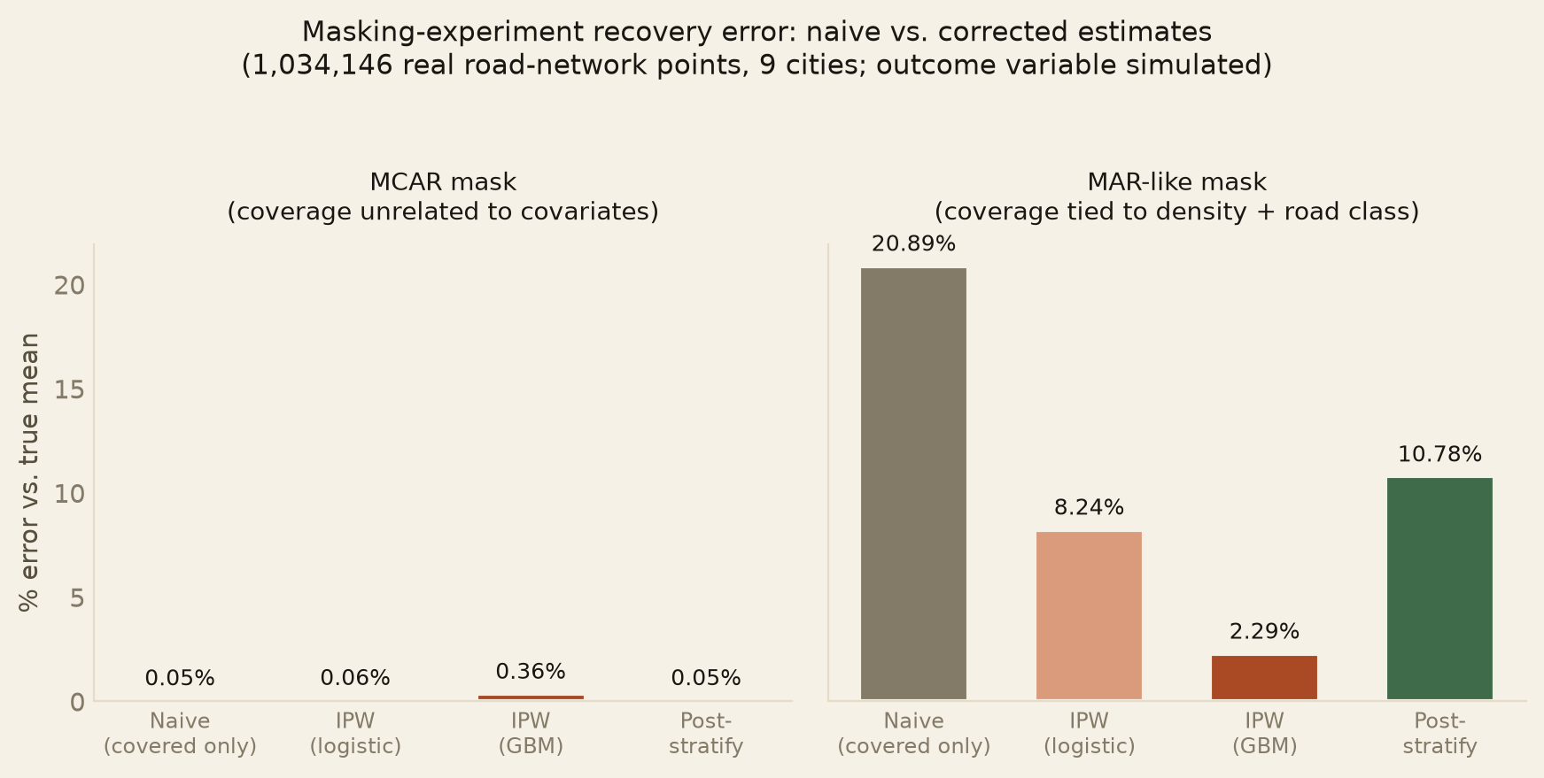
Under MCAR, as expected, every method is close to the true mean — missingness doesn't correlate with the outcome, so there is nothing to fix, and none make things meaningfully worse (all within ~0.4%). Under the MAR-like mechanism, the naive covered-only estimate is substantially biased (20.89% error), because coverage correlates with the same covariates (population density, road importance) that drive the simulated outcome. All three correction methods reduce that bias, but by very different amounts: post-stratification recovers to 10.78% error, logistic-propensity IPW to 8.24%, and gradient-boosted-propensity IPW to 2.29% — the best-recovering method here. This ordering is consistent with the Seaman & White point this project takes seriously: IPW's quality is bounded by the propensity model behind it, and a better-specified (non-linear, gradient-boosted) propensity model recovers substantially more true bias than a linear one fit on identical covariates. This is the one finding this paper can currently report against a known ground truth; it validates the correction methodology, not Indian urban infrastructure or real Mapillary coverage bias.
Robustness
No robustness analysis has been run against real data — there is no real coverage measurement or real infrastructure label yet to run one against. The project's design specifies five robustness axes to check once real data exists: grid size (does the 50m road-sampling spacing materially change coverage or bias estimates versus a coarser or finer spacing), road class (do corrections pooling across road classes hide class-specific coverage mechanisms, e.g. residential streets behaving differently from arterials), spacing/sampling density, model (do the IPW recovery gaps between logistic and gradient-boosted propensity seen here persist, widen, or vanish on real coverage data, where the true mechanism is unknown rather than simulated), and city (does correction effectiveness vary systematically with population tier or economic tier — itself a substantive finding about where this method's assumptions hold least well). The masking experiment offers one weak proxy for the "model" axis — gradient-boosted propensity clearly outperformed logistic under the one mechanism tested — but a single simulated mechanism cannot stand in for a real robustness sweep, and this paper does not claim it does.
Limitations
Data vintage. City populations used for stratified sampling are 2011 Census of India figures, the most recent full national census available (India's 2021 census was postponed and not yet conducted). Cities have grown substantially since 2011, so population-tier stratification reflects a fifteen-year-old snapshot, not current reality. Single-country generalization. Every finding here, real or pending, concerns nine specific Indian cities; nothing generalizes to other Global South urban contexts without independent verification, despite motivating literature (Africa Mapillary coverage, Dollar Street) suggesting the coverage-bias mechanism is not India-specific. Fixed 6km-radius sampling. Necessary to avoid confounding city size with sampling extent (see Data), but it systematically excludes city peripheries for the largest cities in the pool — Mumbai's or Bengaluru's built-up extent reaches well beyond 6km from a single center point, so this project's "urban core" understates true footprint for megacities more than mid-size cities, a residual confound the fixed-radius design does not fully eliminate. VIIRS substitution. Nighttime-lights radiance comes from a peer-reviewed reconstructed dataset (Chen, Wang & Zhang 2024), not the raw NOAA/NCEI distribution, due to an authentication wall in this environment; the 2023 layer is documented as a real annual composite, but it is one processing pipeline removed from the canonical NOAA source and any subtle preprocessing differences are unverified. WorldPop resolution downgrade. Population density is used at 1km rather than the planned 100m, a real precision loss for a covariate whose purpose is discriminating fine-grained density variation within a city. GHSL tile-based approximation. Built-up surface comes from individual 100m tiles selected by a city-center spatial join; a city whose 6km radius straddles a tile boundary could see a subtly discontinuous signal there, not characterized here.
No imagery collected yet is the project's largest limitation: zero Mapillary images queried, zero coverage points measured, zero images labeled, zero vision model trained — every claim about the vision pipeline, cross-city generalization, and real coverage bias in this paper describes implemented, tested, not-yet-executed code, not a result. The masking experiment's outcome is not a real infrastructure signal. infra_quality_index is a deterministic function of real covariates plus noise with realistic-looking structure, not any measured relationship between, say, population density and sidewalk presence — reading its recovery numbers as evidence about real infrastructure-covariate relationships in India would be a category error. Annotation protocol not yet inter-rater-tested. The five-attribute schema and its 10%-overlap double-labeling design have never run against a real image; Cohen's kappa is unknown for every attribute, and it is possible one (building frontage density is the protocol's own flagged candidate) proves too ambiguous for consistent labeling once tested. Economic tier is qualitative, not quantitative — an ordinal label from a consistently-ranked but not numerically-extracted RBI handbook, not a per-capita NSDP figure; anyone treating it as a continuous covariate should pull the real numbers first, which this project explicitly did not do.
Ethics
Street-level imagery of Indian cities, even sourced from a crowdsourced platform under a permissive license, raises genuine privacy concerns: faces, license plates, storefronts, and residences appear incidentally in frame. This project neither downloads nor re-hosts any image bytes — it hotlinks Mapillary's own short-lived thumbnail URLs live from the browser and persists only derived numbers (predictions, confidence, coverage density, propensity scores), a decision documented in docs/data_sources.md specifically to avoid becoming a redistribution point for imagery whose privacy handling is Mapillary's and its contributors' responsibility, not this project's to relitigate.
The more serious risk is representational: any system that scores infrastructure per street segment or neighborhood is one careless dashboard away from ranking neighborhoods "good" or "bad" — a framing this project's own design explicitly refuses to produce. Infrastructure quality correlates with income and caste geography in Indian cities in ways this project has not measured and does not intend to present as a ranking; a public leaderboard of neighborhoods by inferred infrastructure score would risk stigmatization and could be misused to justify disinvestment in already-underserved areas — precisely the population this kind of measurement should serve, not penalize. The coverage-bias half of this project exists specifically because the alternative, treating "where we have imagery" as "how things are," would systematically underrepresent the areas most likely to be under-resourced, compounding rather than correcting existing inequity if used naively.
Relatedly, street-level imagery collection is a mundane form of ambient surveillance infrastructure, and this project is a consumer of it, not a builder — but a system whose purpose is inferring physical conditions from street imagery is one step from repurposing for less benign inference (identifying informal settlements for enforcement rather than investment) if handed to an actor with different incentives. A model whose coverage-bias correction is validated only on a simulated mechanism, and never on real coverage, also carries real risk of confidently mis-correcting once deployed against data whose actual missingness mechanism differs from what was assumed — the Seaman & White caveat emphasized throughout this paper is precisely a warning against that overconfidence. Finally, any eventual use of this project's outputs to inform development policy or infrastructure investment should treat every prediction and bias-corrected estimate as carrying real, unquantified uncertainty; this paper reports point estimates and percent errors from one simulated experiment, not calibrated confidence intervals suitable for a funding decision, and no output here should be the sole basis for one.
Conclusion
UrbanLens India set out to answer two questions: can street-level computer vision measure urban infrastructure in Indian cities, and how biased is that measurement by the uneven availability of the imagery itself. This paper reports honest, partial progress on both. The project's missing-data correction methodology — propensity modeling plus IPW and post-stratification, applied to street-imagery coverage bias with no direct precedent in the literature reviewed here — is validated on a controlled masking experiment built from a real 1,034,146-point Indian road network and real WorldPop/VIIRS/GHSL covariates: naive estimation under a realistic simulated coverage mechanism is 20.89% biased, and a gradient-boosted-propensity IPW correction recovers to 2.29% error. That is a real, if narrowly scoped, methodological contribution. The empirical question this project actually exists to answer — what Indian street infrastructure looks like, how unevenly real imagery captures it, and whether these same correction methods recover an unbiased estimate — remains open, blocked on a single missing dependency: a Mapillary developer API token. Every downstream stage is implemented, unit-tested against synthetic fixtures, and ready to run in order (make coverage, make labels, make train, make bias-study) the moment that token exists. Reporting the project as a completed empirical study of Indian urban infrastructure would misrepresent it; reporting it, as this paper does, as a validated correction methodology on top of a fully built, not-yet-executed measurement pipeline is the accurate description of where it stands.